粗电流环的磁感应分布
目录
⇦
本文上次更新于 1052 天前,其内容可能已经过时,如果文章内容或图片资源失效,请留言反馈,我会及时处理,谢谢!
系统:Windows 10 专业版 1903
matlab版本:Windows版 2018a
使用说明
详细的推导过程见这篇文章, Tokamak_Magnetic.m 为计算磁感应强度的程序, Coarse_Current_Loop.m 为模拟磁感应分布,取消注释和注释掉相关地方,可以画二维和三维图,更改变量choice的值,即可模拟ITER,EAST,HL-2M的极向场分布,如果电流是均匀分布,只需要注释掉 Tokamak_Magnetic.m中电流非均匀分布那一行。
程序
Tokamak_Magnetic.m
function [Bx,By,Bz]=Tokamak_Magnetic(x,y,z)
% 圆截面托卡马克装置,给定某个位置,返回磁场在三个方向的分量
    c0=2e-7;
    %HL-2M
    Ip=3e6;a=0.65;R0=1.78;B0=3.0;
    %ITER
    %Ip=15e6;R0=6.2;a=2.0;B0=5.3;
    rho=sqrt(x^2+y^2);
    theta=atan2(y,x);
    j=Ip/pi/a^2;
    J=@(r,phi)j;       %电流均匀
    J=@(r,phi)J(r,phi)*(1-r.^2./a^2); %电流非均匀
    k2=@(r,phi)4*(R0+r.*cos(phi)).*rho./((R0+r.*cos(phi)+rho).^2+(z-r.*sin(phi)).^2);
    k2=@(r,phi)k2(r,phi)-eps*(k2(r,phi)==1);
    K=@(r,phi)KK(k2(r,phi));
    E=@(r,phi)EE(k2(r,phi));
    dd=@(r,phi)sqrt((R0+r.*cos(phi)+rho).^2+(z-r.*sin(phi)).^2);
    A1=@(r,phi)(R0+r.*cos(phi)).^2+rho^2+(z-r.*sin(phi)).^2;
    A2=@(r,phi)(R0+r.*cos(phi)).^2-rho^2-(z-r.*sin(phi)).^2;
    A3_0=@(r,phi)(R0+r.*cos(phi)-rho).^2+(z-r.*sin(phi)).^2;
    A3=@(r,phi)A3_0(r,phi)+1e-3;        %if A3=0,c/0=inf
    B_rho=@(r,phi)c0*J(r,phi).*r.*(z-r.*sin(phi)).*(A1(r,phi)./A3(r,phi).*E(r,phi)-K(r,phi))./((rho+eps*(rho==0)).*dd(r,phi));
    B_theta=B0*R0/rho;
    B_z=@(r,phi)c0*J(r,phi).*r.*(A2(r,phi)./A3(r,phi).*E(r,phi)+K(r,phi))./dd(r,phi);
    Brho=integral2(B_rho,0,a,0,2*pi);
    Btheta=B_theta;
    Bz=integral2(B_z,0,a,0,2*pi);
    Bx=Brho*cos(theta)-Btheta*sin(theta);
    By=Brho*sin(theta)+Btheta*cos(theta);
end
function K=KK(k2)
    [K,E]=ellipke(k2);
end function E=EE(k2)
    [K,E]=ellipke(k2);
end
Coarse_Current_Loop.m
tic;clc;clear;
global rho z c0 R0 a Ip
c0=2e-7;
%choice=1,EAST,choice=2,ITER,choice=3,HL-2M x1--->rho , x2--> z
choice=3;
switch choice
case 1
a=0.45;R0=1.85;Ip=1e6;
x1=[1:0.02:2.6];x2=linspace(-1,1,length(x1));
case 2
a=2.0;R0=6.2;Ip=15e6;
x1=[3:0.1:9];x2=linspace(-3,3,length(x1));
case 3
a=0.65;R0=1.78;Ip=3e6;
x1=[0.8:0.02:2.6];x2=linspace(-1,1,length(x1));
end
for i1=1:length(x1)
for i2=1:length(x2)
z=x2(i2);
rho=x1(i1);
Brho=integral2(@whatBrho,0,a,0,2*pi);
Bz=integral2(@whatBz,0,a,0,2*pi);
B(i1,i2)=sqrt(Brho^2+Bz^2);
end
end
%二维图
plot(x1,B);
xlabel(['\fontname{Arial}R']);
ylabel(['\fontname{Arial}Bp']);
%zlabel(['\fontname{Arial}z']);
set(gca,'FontSize',20);
%三维图
% mesh(x1,x2,B');
% axis tight;
%xlabel(['\fontname{Arial}R']);
%ylabel(['\fontname{Arial}Z']);
%zlabel(['\fontname{Arial}Bp']);
% set(gca,'FontSize',20); %set axis size
% disp(['calculation time ' num2str(toc) 's']);
% savefiles(choice);
% disp(['total time ' num2str(toc) 's']);
function B_rho=whatBrho(r,theta)
global c0 z rho
[A1,~,A3,dd,J,E,K]=parameter(r,theta);
B_rho=c0*J.*r.*(z-r.*sin(theta)).*(A1./A3.*E-K)./(rho*dd);
end
function B_z=whatBz(r,theta)
global c0
[~,A2,A3,dd,J,E,K]=parameter(r,theta);
B_z=c0*J.*r.*(A2./A3.*E+K)./dd;
end
%计算过程中定义的一些参数
function [A1,A2,A3,dd,J,E,K]=parameter(r,theta)
% theta为截面的,不是柱坐标下的theta,r也不是柱坐标下的r
global rho z a R0 Ip
J=Ip/pi/a^2; %dian liu jun yun
%J=J*(1-r.^2./a^2); %fei jun yun
%修改后的R,Z,圆截面
R=R0+r.*cos(theta);
Z=z-r.*sin(theta);
%等离子体截面非圆,某些参数与r有关
%R=R0-b+(a+b*cos(theta))*cos(theta+delta*sin(theta));
%Z=k*a*sin(theta);
k2=4*R*rho./((R+rho).^2+Z.^2);
k2=k2-eps;
[K,E]=ellipke(k2);
dd=sqrt((R+rho).^2+Z.^2);
A1=R.^2+rho^2+Z.^2;
A2=R.^2-rho^2-Z.^2;
A3=(R-rho).^2+Z.^2;
A3=A3+1e-3; %避免分母出现零
end
function savefiles(choice)
time=datestr(now,30);
switch choice
case 1
print(gcf,['Coarse_Current_Loop_EAST_',time,'.eps'],'-depsc','-r600')
savefig(['Coarse_Current_Loop_EAST_',time,'.fig'])
print(gcf,['Coarse_Current_Loop_EAST_',time,'.png'],'-dpng')
case 2
print(gcf,['Coarse_Current_Loop_ITER_',time,'.eps'],'-depsc','-r600')
savefig(['Coarse_Current_Loop_ITER_',tme,'.fig'])
print(gcf,['Coarse_Current_Loop_ITER_',time,'.png'],'-dpng')
case 3
print(gcf,['Coarse_Current_Loop_HL_2M_',time,'.eps'],'-depsc','-r600')
savefig(['Coarse_Current_Loop_HL_2M_',time,'.fig'])
print(gcf,['Coarse_Current_Loop_HL_2M_',time,'.png'],'-dpng')
end
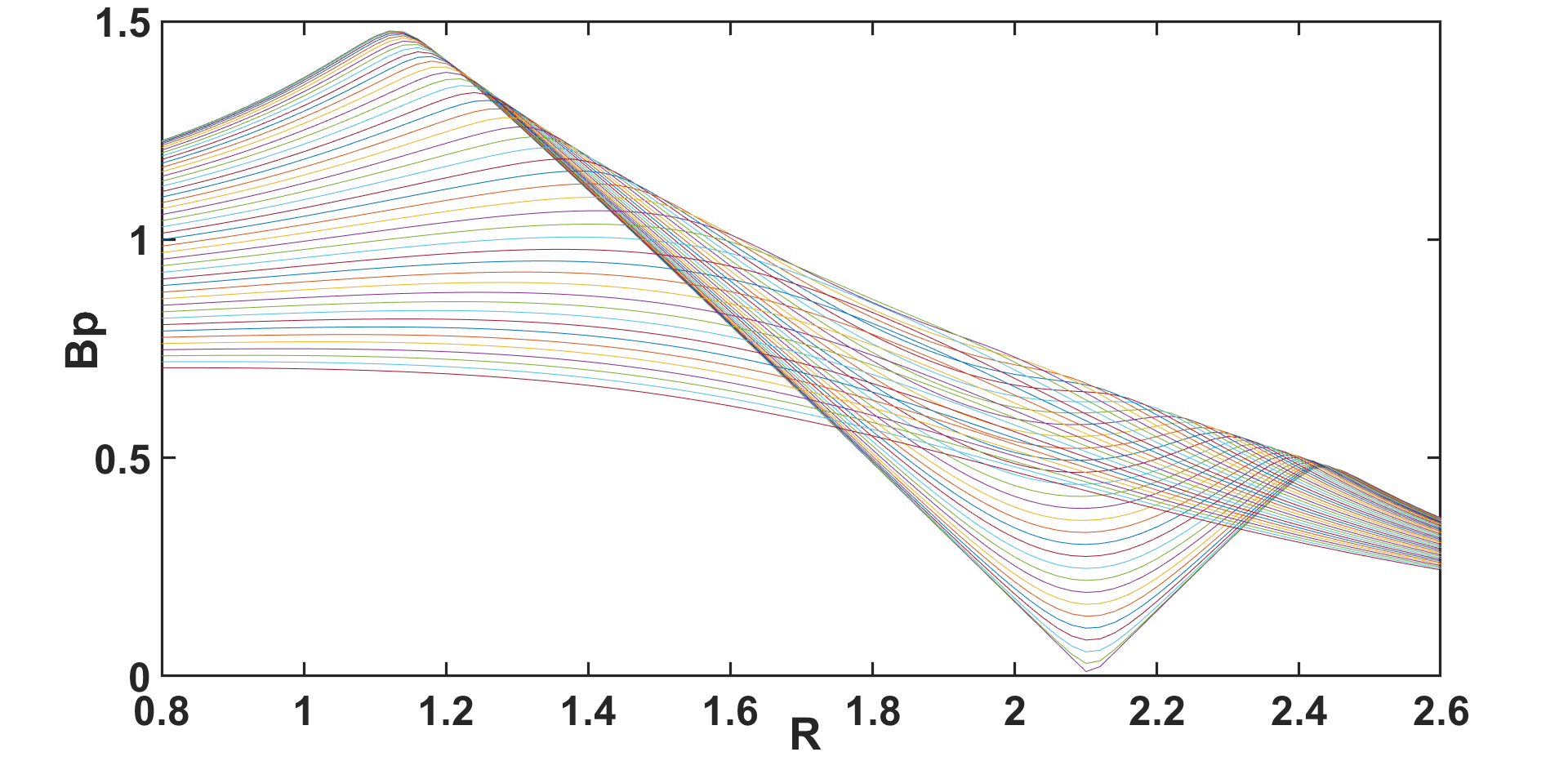
end取choice=3得到的结果,二维图,电流均匀
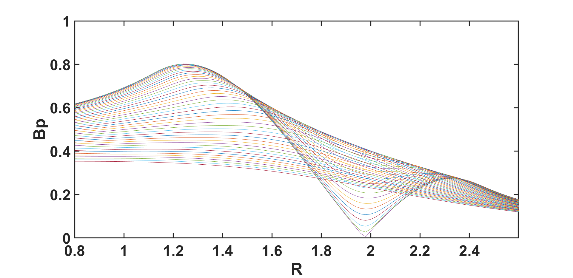
取choice=3得到的结果,二维图,电流非均匀
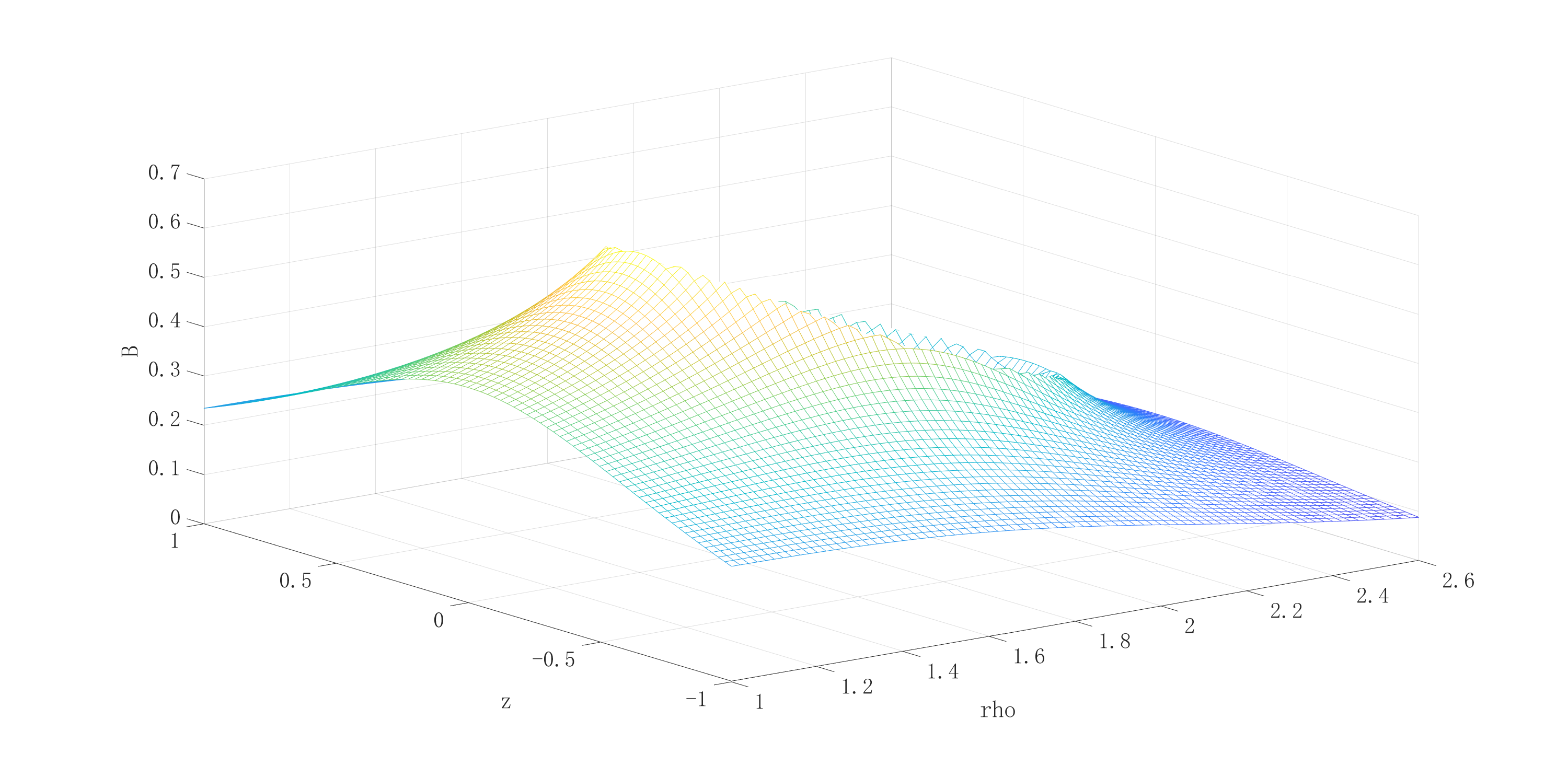
取choice=1时,得到的结果(需要注释掉程序中的画二维图,取消注释程序中的画三维图),运行大约需要100多秒。
源码
如果在这个过程中遇到了其它问题,欢迎在评论区留言,如果你已解决,也欢迎把具体的解决方法留在评论区,以供后来者参考
×


感谢您的支持,请扫码打赏